
Passing a Chicken through an MNIST Model
When you put a picture of a chicken through a model trained on MNIST, the model is 99.9% confident that the chicken is a 5. That’s not good.
This problem does not just relate to chickens and digits but the fact that a neural net makes very confident predictions on data that does not come from the same distribution as the training data. While this example is artificial, it is common in practice for a machine learning model to be used on data that is very different from the data it was trained on. A self-driving car, for example, may encounter an unusual environment that was never seen during training. In such cases, the system should not be overly confident but instead let the driver know that it is not able to make a meaningful prediction.1
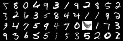
Images from MNIST and a chicken.
Discriminative models and unseen data
When doing classification we are often interested in building a discriminative model \(p(y \vert x)\), i.e. a model of the probability of a certain label \(y\) (e.g. digit type) given a datapoint \(x\) (e.g. an image of a digit). If we use data drawn from a distribution \(p_{\text{train}}(x)\) to train a discriminative model \(p(y \vert x)\), how will the trained model behave when we input an \(x\) that is very far from \(p_{\text{train}}(x)\)? For example, if we train a model to predict digit type from an image of a digit, what happens when we put a picture of a chicken through this model?
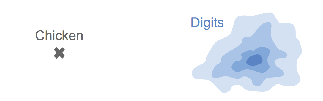
In the space of images, chickens lie far away from digits. This figure shows the distribution of digits in blue (corresponding to the training distribution in our case) and where an image of a chicken would lie relative to this.
Chicken probabilities under an MNIST model
To explore these problems, we train a simple convolutional neural network (CNN) on MNIST which gets about 98% testing accuracy. We would then like to see what happens to the output probabilities \(p(y \vert x)\) of the trained model when shown images that are completely different from digits. As an example, we pass an “MNIST-ified” chicken through the model.2
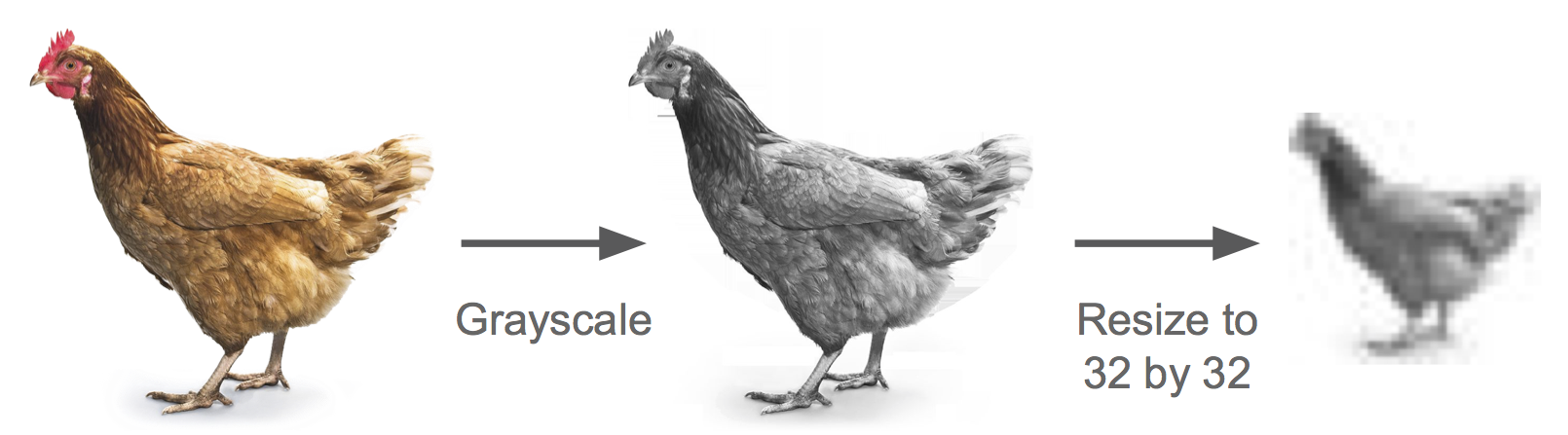
An MNIST-ified chicken. The CNN takes in 32 by 32 grayscale images, so we transform the image of the chicken to match this.
Ideally, the outputs \(p(y \vert x)\) would be approximately uniform, i.e. the probability of every class would be about 10%. This would mean that the CNN has little confidence that the chicken belongs to any of the 10 classes. However, for the above picture of a chicken, the probability of the label 5 is 99.9%.
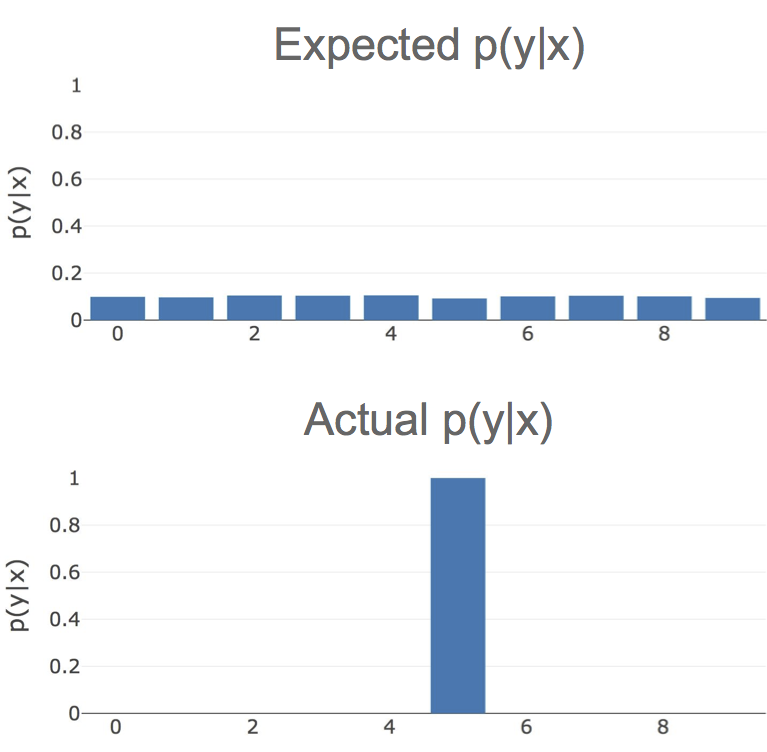
Histograms of expected vs actual softmax class probabilities for an image of a chicken on an MNIST model.
The model is extremely confident that this chicken is the digit 5 even though, to a human, it clearly isn’t. Even worse, it is much more confident that this chicken is a 5 than many other digits that are actually a 5.
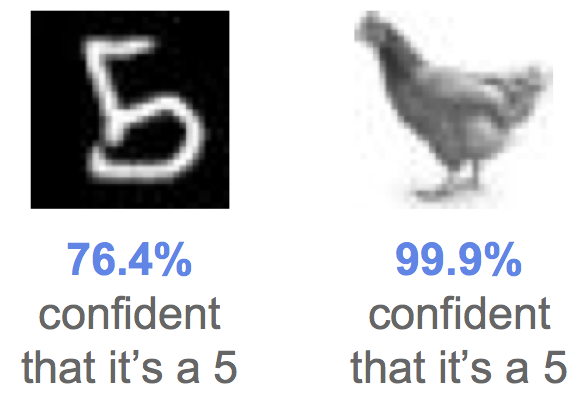
The model is more confident that the image on the right is a 5 than the image on the left.
Fashion probabilities under an MNIST model
Of course, it could be that this image of a chicken is just a fluke and high confidence predictions for data outside of \(p_{\text{train}}(x)\) are rare. To test this, we use the FashionMNIST dataset which contains images of various types clothing.
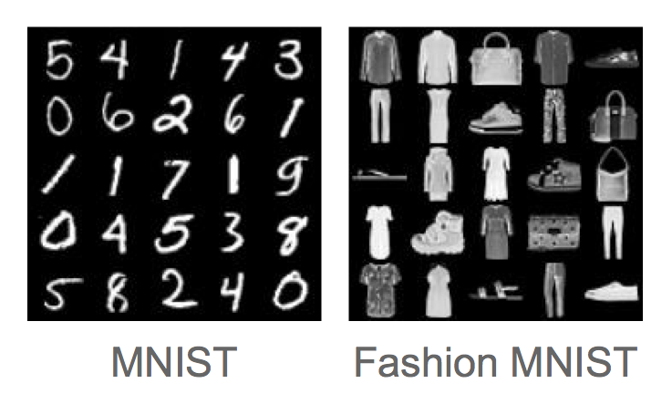
MNIST and FashionMNIST examples. The images are the same size and both contain 10 classes.
These images have nothing to do with digits, so again we would hope that the model will only make low confidence predictions. We predict \(p(y \vert x)\) for 10000 images from the Fashion MNIST dataset using the trained MNIST model and measure the fraction of them which have a high confidence prediction (i.e. where the maximum probability of a certain class \(\max_y p(y \vert x)\) is very high). The results are shown below:
- 63.4% of examples have more than 99% confidence
- 74.3% of examples have more than 95% confidence
- 88.9% of examples have more than 75% confidence
Almost two thirds of the Fashion MNIST dataset is classified as a certain digit type with more than 99% confidence. This shows that neural nets can consistently make confident predictions about unseen data and that using the output probabilities as a measure of confidence does not make much sense, at least on data that is very far from the training data.
We can also look at how confident3 predictions on the fashion items are compared to those on correctly classified digits. To do this, we draw a vertical pink line for every FashionMNIST image and a blue line for every MNIST image. We then sort the lines by the confidence of the prediction on the corresponding image. Ideally, the resulting plot would be all pink on the left and all blue on the right (i.e all MNIST examples have higher confidence than the FashionMNIST examples under an MNIST model). The actual results are shown below.

Images sorted by confidence. The x-axis corresponds to increasing confidence and each vertical line to an image.
Ideally, all FashionMNIST images would have lower confidence and so be on the left, but this is not the case.
Natural adversarial examples
The chicken and fashion images can loosely be thought of as “natural” adversarial examples. Adversarial examples are typically images from a certain class (e.g. 5) that have been imperceptibly modified to be misclassified as another class (e.g. 7) with high confidence. In the same way that adversarial examples fool the machine learning model, the chicken and fashion images “fool” the model into classifying these images into a certain class with high confidence even though they do not belong to that class (or any of the classes in our case). Machine Learning systems should not only be protected from attackers that maliciously modify images but also from naturally occurring images that are far from the training distribution.
Modeling the data p(x)
It seems clear that we can’t solely rely on modeling \(p(y \vert x)\) when data far from \(p_{\text{train}}(x)\) may be used at test time. In the real world, it is often very difficult to constrain the user only to use data drawn from \(p_{\text{train}}(x)\).
One way to solve this problem is to not only model \(p(y \vert x)\) but to also model \(p_{\text{train}}(x)\). If we can model \(p_{\text{train}}(x)\) and we get a new sample \(x_{\text{test}}\), we can first check whether this sample is probable under \(p_{\text{train}}(x)\). If it is, we have seen something similar before so we should go ahead and predict \(p(y \vert x)\), otherwise we can reject this sample.
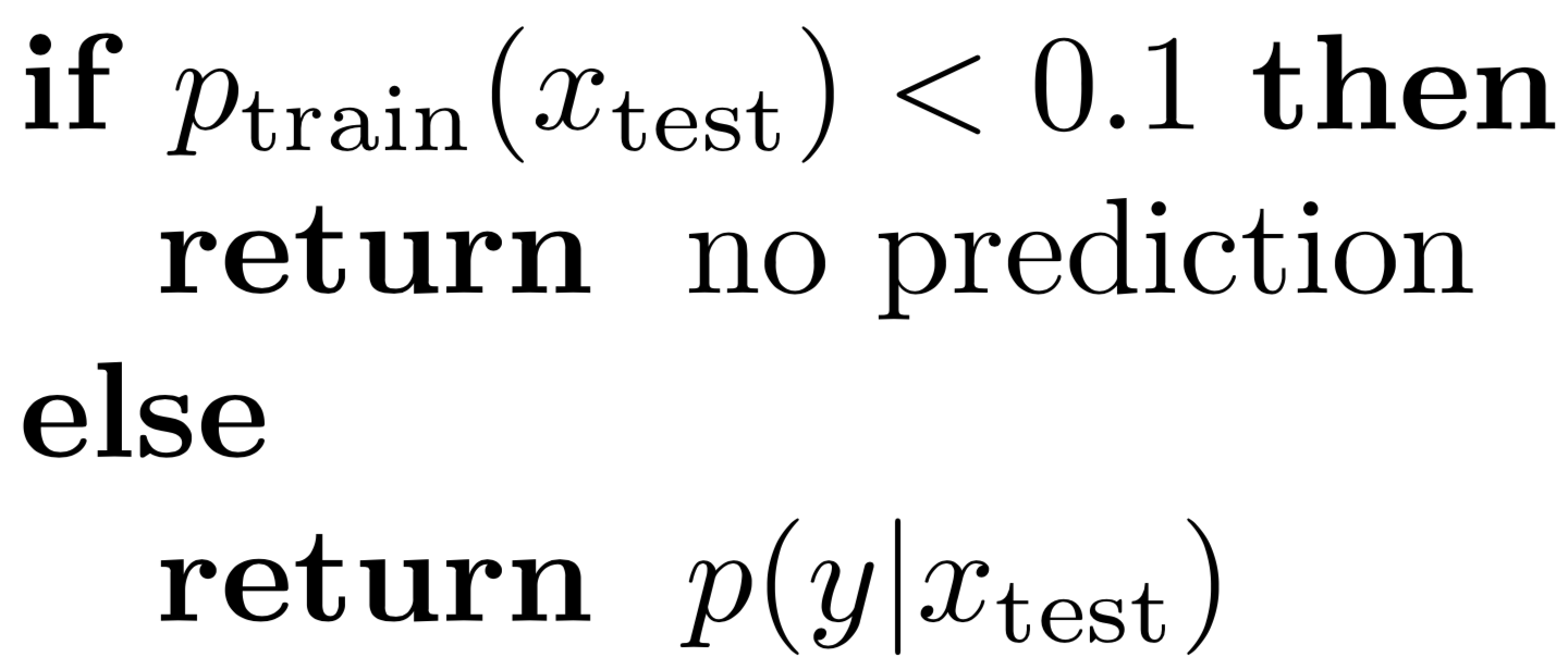
Simple algorithm for returning meaningful predictions.
There are several ways of modeling p(x). In this post, we will focus on variational autoencoders (VAE) which have been quite successful at modeling distributions of images.
Variational Autoencoders to model p(x)
VAEs are generative models that learn a joint model \(p(x, z)\) of the data \(x\) and some latent variables \(z\). As the name suggests, VAEs are closely related to autoencoders. VAEs work by encoding a datapoint \(x\) into a distribution \(q(z \vert x)\) of latent variables and then sampling a latent vector \(z\) from this distribution. The sample \(z\) is then decoded into a reconstruction of the encoded data \(x\). The encoder and decoder are typically neural networks.
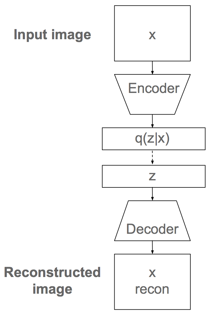
Sketch of VAE architecture, sampling is shown with dashed lines.
Interestingly, VAEs optimize a lower bound on \(\log p(x)\) called the Evidence Lower Bound (ELBO).
\[\log p(x) >= \text{ELBO} = - \text{VAE loss}\]So after training a VAE on data from \(p_{\text{train}}\), we can calculate the loss on a new example \(x_{\text{test}}\) and obtain a lower bound on the log likelihood of that example under \(p_{\text{train}}\). Of course, this is a lower bound, but the hope is that for a well trained model, this lower bound is fairly tight.
Reconstruction of a digit and a chicken
To test this, we train a convolutional VAE on MNIST. Note that the ELBO is the sum of a reconstruction error term and a KL divergence term. So if an image is poorly reconstructed by the VAE, it will typically have low probability. The figure below shows reconstructions from the trained VAE.
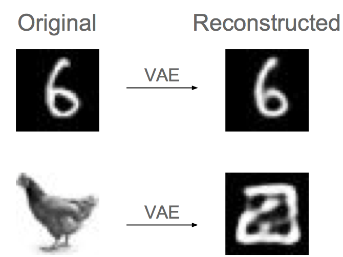
A digit and a chicken reconstructed by a VAE trained on MNIST. As can be seen the digit is well reconstructed while the chicken is not. This suggests the chicken has low probability under the training distribution.
We can now use the VAE to predict the probability of 10000 FashionMNIST images and 10000 MNIST images under \(p_{\text{train}}\). Ideally, the probabilities of FashionMNIST examples would be considerably lower than all the MNIST examples and we would get a good separation between the two. The figure below shows the results, with sorted probabilities from lowest to highest.

FashionMNIST and MNIST examples sorted by probabilities from a VAE model.
As can be seen the separation is much cleaner than when using the maximum class probabilities \(p(y \vert x)\). This shows that modeling \(p(x)\) can be useful for classification tasks when data different from the training data may be used at test time.
Conclusion
In this post we used the toy example of chickens and digits to show that a deep learning model can make confident, but meaningless, predictions on data it has never seen. Not only does a chicken get confidently classified as a 5 by an MNIST model, other natural images such as fashion items consistently fool the classifier into making high confidence predictions. We showed that modeling \(p(x)\) with a VAE is a simple solution that can partially mitigate this problem. However, solving this problem and, more generally, modeling uncertainty in deep learning is an important area of research.
Footnotes
1. The idea of putting a picture of a chicken through an MNIST model initially came from a question I heard on the Approximate Inference panel at NIPS 2017
2. I resized MNIST from 28 by 28 to 32 by 32 for these experiments
3. The word confidence is used loosely here and is not related to confidence in the statistical sense. However \(\max_y p(y \vert x)\) is commonly used to show that a model is “confident” about its predictions and this is how we use it here